

Customer Churn Prediction using PySpark
Binary Customer Churn Evaluator
Use Case
A marketing agency has many customers that use their service to produce ads for the client/customer websites.They’ve noticed that they have quite a bit of churn in clients. They basically randomly assign account managers right now, but want me to create a machine learning model that will help predict which customers will churn (stop buying their service) so that they can correctly assign the customers most at risk to churn an account manager. Luckily they have some historical data. I have created a classification algorithm that will help classify whether or not a customer churned. Then the company can test this against incoming data for future customers to predict which customers will churn and assign them an account manager.
The data is saved as customer_churn.csv. Here are the fields and their definitions:
Name : Name of the latest contact at Company
Age: Customer Age
Total_Purchase: Total Ads Purchased
Account_Manager: Binary 0=No manager, 1= Account manager assigned
Years: Totaly Years as a customer
Num_sites: Number of websites that use the service.
Onboard_date: Date that the name of the latest contact was onboarded
Location: Client HQ Address
Company: Name of Client Company
Once we’ve created the model and evaluated it, we have to test out the model on some new data that your client has provided, saved under new_customers.csv. The client wants to know which customers are most likely to churn given this data (they don’t have the label yet).
import findspark
findspark.init('/home/ubuntu/spark-2.1.1-bin-hadoop2.7')
import pyspark
from pyspark.sql import SparkSession
spark = SparkSession.builder.appName('Churn').getOrCreate()
from pyspark.ml.classification import LogisticRegression
from pyspark.ml.feature import VectorAssembler
from pyspark.ml.evaluation import BinaryClassificationEvaluator
import matplotlib.pyplot as plt
import seaborn as sns
import pandas as pd
import numpy as np
df = spark.read.csv('customer_churn.csv',inferSchema=True,header=True)
Print Schema of the Spark Dataframe
df.printSchema()
root
 |-- Names: string (nullable = true)
 |-- Age: integer (nullable = true)
 |-- Total_Purchase: double (nullable = true)
 |-- Account_Manager: integer (nullable = true)
 |-- Years: double (nullable = true)
 |-- Num_Sites: integer (nullable = true)
 |-- Onboard_date: string (nullable = true)
 |-- Location: string (nullable = true)
 |-- Company: string (nullable = true)
 |-- Churn: integer (nullable = true)
Print Column Names
df.columns
['Names',
 'Age',
 'Total_Purchase',
 'Account_Manager',
 'Years',
 'Num_Sites',
 'Onboard_date',
 'Location',
 'Company',
 'Churn']
df.describe().show()
+-------+-------------+-----------------+-----------------+------------------+-----------------+------------------+----------------+--------------------+--------------------+-------------------+
|summary|        Names|              Age|   Total_Purchase|   Account_Manager|            Years|         Num_Sites|    Onboard_date|            Location|             Company|              Churn|
+-------+-------------+-----------------+-----------------+------------------+-----------------+------------------+----------------+--------------------+--------------------+-------------------+
|  count|          900|              900|              900|               900|              900|               900|             900|                 900|                 900|                900|
|   mean|         null|41.81666666666667|10062.82403333334|0.4811111111111111| 5.27315555555555| 8.587777777777777|            null|                null|                null|0.16666666666666666|
| stddev|         null|6.127560416916251|2408.644531858096|0.4999208935073339|1.274449013194616|1.7648355920350969|            null|                null|                null| 0.3728852122772358|
|    min|   Aaron King|               22|            100.0|                 0|              1.0|                 3|01-01-2012 21:48|00103 Jeffrey Cre...|     Abbott-Thompson|                  0|
|    max|Zachary Walsh|               65|         18026.01|                 1|             9.15|                14|31-10-2014 16:00|Unit 9800 Box 287...|Zuniga, Clark and...|                  1|
+-------+-------------+-----------------+-----------------+------------------+-----------------+------------------+----------------+--------------------+--------------------+-------------------+
df.show(10)
+----------------+---+--------------+---------------+-----+---------+----------------+--------------------+--------------------+-----+
|           Names|Age|Total_Purchase|Account_Manager|Years|Num_Sites|    Onboard_date|            Location|             Company|Churn|
+----------------+---+--------------+---------------+-----+---------+----------------+--------------------+--------------------+-----+
|Cameron Williams| 42|       11066.8|              0| 7.22|        8|30-08-2013 07:00|10265 Elizabeth M...|          Harvey LLC|    1|
|   Kevin Mueller| 41|      11916.22|              0|  6.5|       11|13-08-2013 00:38|6157 Frank Garden...|          Wilson PLC|    1|
|     Eric Lozano| 38|      12884.75|              0| 6.67|       12|29-06-2016 06:20|1331 Keith Court ...|Miller, Johnson a...|    1|
|   Phillip White| 42|       8010.76|              0| 6.71|       10|22-04-2014 12:43|13120 Daniel Moun...|           Smith Inc|    1|
|  Cynthia Norton| 37|       9191.58|              0| 5.56|        9|19-01-2016 15:31|765 Tricia Row Ka...|          Love-Jones|    1|
|Jessica Williams| 48|      10356.02|              0| 5.12|        8|03-03-2009 23:13|6187 Olson Mounta...|        Kelly-Warren|    1|
|     Eric Butler| 44|      11331.58|              1| 5.23|       11|05-12-2016 03:35|4846 Savannah Roa...|   Reynolds-Sheppard|    1|
|   Zachary Walsh| 32|       9885.12|              1| 6.92|        9|09-03-2006 14:50|25271 Roy Express...|          Singh-Cole|    1|
|     Ashlee Carr| 43|       14062.6|              1| 5.46|       11|29-09-2011 05:47|3725 Caroline Str...|           Lopez PLC|    1|
|  Jennifer Lynch| 40|       8066.94|              1| 7.11|       11|28-03-2006 15:42|363 Sandra Lodge ...|       Reed-Martinez|    1|
+----------------+---+--------------+---------------+-----+---------+----------------+--------------------+--------------------+-----+
only showing top 10 rows
Vector assembler’s job is to combine the raw features and features generated from various transforms into a single feature vector.
assembler = VectorAssembler(inputCols=['Age',
 'Total_Purchase',
 'Account_Manager',
 'Years',
 'Num_Sites'],outputCol='features')
output = assembler.transform(df)
final_data = output.select('features','churn')
final_data.show()
+--------------------+-----+
|            features|churn|
+--------------------+-----+
|[42.0,11066.8,0.0...|    1|
|[41.0,11916.22,0....|    1|
|[38.0,12884.75,0....|    1|
|[42.0,8010.76,0.0...|    1|
|[37.0,9191.58,0.0...|    1|
|[48.0,10356.02,0....|    1|
|[44.0,11331.58,1....|    1|
|[32.0,9885.12,1.0...|    1|
|[43.0,14062.6,1.0...|    1|
|[40.0,8066.94,1.0...|    1|
|[30.0,11575.37,1....|    1|
|[45.0,8771.02,1.0...|    1|
|[45.0,8988.67,1.0...|    1|
|[40.0,8283.32,1.0...|    1|
|[41.0,6569.87,1.0...|    1|
|[38.0,10494.82,1....|    1|
|[45.0,8213.41,1.0...|    1|
|[43.0,11226.88,0....|    1|
|[53.0,5515.09,0.0...|    1|
|[46.0,8046.4,1.0,...|    1|
+--------------------+-----+
only showing top 20 rows
Splitting the data into training and testing data
train_churn,test_churn = final_data.randomSplit([0.7,0.3])
Logistic Regression
lr_churn = LogisticRegression(featuresCol = 'features',labelCol='churn')
fitted_churn_model = lr_churn.fit(train_churn)
training_sum = fitted_churn_model.summary
Evaluate results
Let’s evaluate the results on the data set we were given (using the test data)
pred_and_labels = fitted_churn_model.evaluate(test_churn)
pred_and_labels.predictions.show()
+--------------------+-----+--------------------+--------------------+----------+
|            features|churn|       rawPrediction|         probability|prediction|
+--------------------+-----+--------------------+--------------------+----------+
|[22.0,11254.38,1....|    0|[5.52159691806313...|[0.99601647589334...|       0.0|
|[28.0,9090.43,1.0...|    0|[1.98633570663306...|[0.87935493331968...|       0.0|
|[28.0,11245.38,0....|    0|[4.30633075424808...|[0.9866964398551,...|       0.0|
|[29.0,5900.78,1.0...|    0|[4.96690245369377...|[0.99308348328094...|       0.0|
|[29.0,8688.17,1.0...|    1|[3.29103080746525...|[0.96411982968159...|       0.0|
|[29.0,9617.59,0.0...|    0|[5.09436401487799...|[0.99390615784382...|       0.0|
|[29.0,10203.18,1....|    0|[4.42382577320060...|[0.98815373632693...|       0.0|
|[29.0,11274.46,1....|    0|[5.16168197118429...|[0.99430061871156...|       0.0|
|[30.0,8403.78,1.0...|    0|[6.84447297381239...|[0.99893580617074...|       0.0|
|[30.0,8677.28,1.0...|    0|[4.91135208556190...|[0.99269128378697...|       0.0|
|[30.0,11575.37,1....|    1|[4.56388496720454...|[0.98968599430140...|       0.0|
|[30.0,13473.35,0....|    0|[2.95897473235687...|[0.95068594934318...|       0.0|
|[31.0,8829.83,1.0...|    0|[5.13438230311274...|[0.99414380796431...|       0.0|
|[31.0,10182.6,1.0...|    0|[5.46281214650561...|[0.99577630434757...|       0.0|
|[31.0,11297.57,1....|    1|[1.20390876464038...|[0.76921940104325...|       0.0|
|[31.0,11743.24,0....|    0|[7.50618051206994...|[0.99945062541098...|       0.0|
|[31.0,12264.68,1....|    0|[4.00916951245971...|[0.98217503463885...|       0.0|
|[32.0,5756.12,0.0...|    0|[4.90586880426166...|[0.99265139327543...|       0.0|
|[32.0,6367.22,1.0...|    0|[3.58538447261660...|[0.97302198685523...|       0.0|
|[32.0,8617.98,1.0...|    1|[1.36636436550272...|[0.79679212701404...|       0.0|
+--------------------+-----+--------------------+--------------------+----------+
only showing top 20 rows
Using Binary Classification Evaluator to evaluate our results
churn_eval = BinaryClassificationEvaluator(rawPredictionCol='prediction',
                                           labelCol='churn')
auc = churn_eval.evaluate(pred_and_labels.predictions)
auc
0.7764291670527194
from sklearn.metrics import roc_curve, roc_auc_score
test_lr_model = fitted_churn_model.transform(test_churn)
test_lr_model.show()
+--------------------+-----+--------------------+--------------------+----------+
|            features|churn|       rawPrediction|         probability|prediction|
+--------------------+-----+--------------------+--------------------+----------+
|[22.0,11254.38,1....|    0|[5.52159691806313...|[0.99601647589334...|       0.0|
|[28.0,9090.43,1.0...|    0|[1.98633570663306...|[0.87935493331968...|       0.0|
|[28.0,11245.38,0....|    0|[4.30633075424808...|[0.9866964398551,...|       0.0|
|[29.0,5900.78,1.0...|    0|[4.96690245369377...|[0.99308348328094...|       0.0|
|[29.0,8688.17,1.0...|    1|[3.29103080746525...|[0.96411982968159...|       0.0|
|[29.0,9617.59,0.0...|    0|[5.09436401487799...|[0.99390615784382...|       0.0|
|[29.0,10203.18,1....|    0|[4.42382577320060...|[0.98815373632693...|       0.0|
|[29.0,11274.46,1....|    0|[5.16168197118429...|[0.99430061871156...|       0.0|
|[30.0,8403.78,1.0...|    0|[6.84447297381239...|[0.99893580617074...|       0.0|
|[30.0,8677.28,1.0...|    0|[4.91135208556190...|[0.99269128378697...|       0.0|
|[30.0,11575.37,1....|    1|[4.56388496720454...|[0.98968599430140...|       0.0|
|[30.0,13473.35,0....|    0|[2.95897473235687...|[0.95068594934318...|       0.0|
|[31.0,8829.83,1.0...|    0|[5.13438230311274...|[0.99414380796431...|       0.0|
|[31.0,10182.6,1.0...|    0|[5.46281214650561...|[0.99577630434757...|       0.0|
|[31.0,11297.57,1....|    1|[1.20390876464038...|[0.76921940104325...|       0.0|
|[31.0,11743.24,0....|    0|[7.50618051206994...|[0.99945062541098...|       0.0|
|[31.0,12264.68,1....|    0|[4.00916951245971...|[0.98217503463885...|       0.0|
|[32.0,5756.12,0.0...|    0|[4.90586880426166...|[0.99265139327543...|       0.0|
|[32.0,6367.22,1.0...|    0|[3.58538447261660...|[0.97302198685523...|       0.0|
|[32.0,8617.98,1.0...|    1|[1.36636436550272...|[0.79679212701404...|       0.0|
+--------------------+-----+--------------------+--------------------+----------+
only showing top 20 rows
dfg = test_lr_model.toPandas()
AUROC = roc_auc_score(dfg['churn'],dfg['prediction'])
AUROC
0.7764291670527194
dfg.head(10)
| features | churn | rawPrediction | probability | prediction | |
|---|---|---|---|---|---|
| 0 | [22.0, 11254.38, 1.0, 4.96, 8.0] | 0 | [5.521596918063132, -5.521596918063132] | [0.9960164758933467, 0.0039835241066532405] | 0.0 |
| 1 | [28.0, 9090.43, 1.0, 5.74, 10.0] | 0 | [1.9863357066330636, -1.9863357066330636] | [0.8793549333196816, 0.12064506668031845] | 0.0 |
| 2 | [28.0, 11245.38, 0.0, 6.72, 8.0] | 0 | [4.30633075424808, -4.30633075424808] | [0.9866964398551, 0.013303560144900025] | 0.0 |
| 3 | [29.0, 5900.78, 1.0, 5.56, 8.0] | 0 | [4.966902453693777, -4.966902453693777] | [0.993083483280944, 0.006916516719056102] | 0.0 |
| 4 | [29.0, 8688.17, 1.0, 5.7, 9.0] | 1 | [3.2910308074652583, -3.2910308074652583] | [0.9641198296815964, 0.035880170318403674] | 0.0 |
| 5 | [29.0, 9617.59, 0.0, 5.49, 8.0] | 0 | [5.094364014877996, -5.094364014877996] | [0.9939061578438267, 0.006093842156173179] | 0.0 |
| 6 | [29.0, 10203.18, 1.0, 5.82, 8.0] | 0 | [4.423825773200608, -4.423825773200608] | [0.9881537363269345, 0.011846263673065542] | 0.0 |
| 7 | [29.0, 11274.46, 1.0, 4.43, 8.0] | 0 | [5.16168197118429, -5.16168197118429] | [0.9943006187115672, 0.005699381288432765] | 0.0 |
| 8 | [30.0, 8403.78, 1.0, 4.13, 7.0] | 0 | [6.844472973812392, -6.844472973812392] | [0.9989358061707416, 0.0010641938292584945] | 0.0 |
| 9 | [30.0, 8677.28, 1.0, 7.31, 7.0] | 0 | [4.911352085561905, -4.911352085561905] | [0.9926912837869708, 0.007308716213029219] | 0.0 |
dfg.describe()
| churn | prediction | |
|---|---|---|
| count | 294.000000 | 294.000000 |
| mean | 0.146259 | 0.132653 |
| std | 0.353968 | 0.339778 |
| min | 0.000000 | 0.000000 |
| 25% | 0.000000 | 0.000000 |
| 50% | 0.000000 | 0.000000 |
| 75% | 0.000000 | 0.000000 |
| max | 1.000000 | 1.000000 |
a=[]
for i in range(294):
    a.append(dfg['probability'][i][1])
dft = pd.DataFrame(a)
dft.columns = ['Probability of not churn']
dft.head(10)
| Probability of not churn | |
|---|---|
| 0 | 0.003984 |
| 1 | 0.120645 |
| 2 | 0.013304 |
| 3 | 0.006917 |
| 4 | 0.035880 |
| 5 | 0.006094 |
| 6 | 0.011846 |
| 7 | 0.005699 |
| 8 | 0.001064 |
| 9 | 0.007309 |
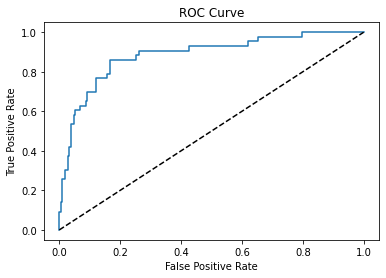
fpr,tpr,thresholds = roc_curve(dfg['churn'],dft['Probability of not churn'])
plt.plot(fpr,tpr)
plt.plot(fpr,fpr,linestyle='--',color='k')
plt.xlabel('False Positive Rate')
plt.ylabel('True Positive Rate')
plt.title('ROC Curve')
Text(0.5, 1.0, 'ROC Curve')
from sklearn.metrics import plot_confusion_matrix
dfg.head(10)
| features | churn | rawPrediction | probability | prediction | |
|---|---|---|---|---|---|
| 0 | [25.0, 9672.03, 0.0, 5.49, 8.0] | 0 | [5.058411246307447, -5.058411246307447] | [0.9936844901076958, 0.006315509892304134] | 0.0 |
| 1 | [26.0, 8939.61, 0.0, 4.54, 7.0] | 0 | [6.91156995401764, -6.91156995401764] | [0.9990047988204478, 0.0009952011795522138] | 0.0 |
| 2 | [29.0, 11274.46, 1.0, 4.43, 8.0] | 0 | [4.5384903283838725, -4.5384903283838725] | [0.9894235255017542, 0.010576474498245805] | 0.0 |
| 3 | [29.0, 13255.05, 1.0, 4.89, 8.0] | 0 | [4.121378406981179, -4.121378406981179] | [0.984036818621191, 0.01596318137880903] | 0.0 |
| 4 | [30.0, 8403.78, 1.0, 4.13, 7.0] | 0 | [6.220715534045645, -6.220715534045645] | [0.998016121244835, 0.0019838787551648912] | 0.0 |
| 5 | [30.0, 10183.98, 1.0, 5.14, 9.0] | 0 | [2.8533233218640888, -2.8533233218640888] | [0.9454902154988308, 0.05450978450116926] | 0.0 |
| 6 | [30.0, 10960.52, 1.0, 5.96, 9.0] | 0 | [2.34321738025276, -2.34321738025276] | [0.912393596720317, 0.08760640327968308] | 0.0 |
| 7 | [30.0, 12788.37, 0.0, 4.31, 10.0] | 0 | [2.4729410654229937, -2.4729410654229937] | [0.922222983019071, 0.077777016980929] | 0.0 |
| 8 | [30.0, 13473.35, 0.0, 3.84, 10.0] | 0 | [2.6695317343018417, -2.6695317343018417] | [0.935204661724413, 0.06479533827558702] | 0.0 |
| 9 | [31.0, 5304.6, 0.0, 5.29, 9.0] | 0 | [3.8526638669261573, -3.8526638669261573] | [0.9792179348879895, 0.020782065112010563] | 0.0 |
from sklearn import metrics
import pandas as pd
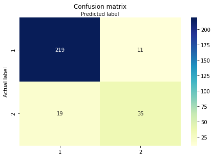
cnf_matrix = metrics.confusion_matrix(dfg['churn'], dfg['prediction'])
class_names=[1,2,3,4,5] # name  of classes
fig, ax = plt.subplots()
# create heatmap
sns.heatmap(pd.DataFrame(cnf_matrix), annot=True, cmap="YlGnBu" ,fmt='g')
ax.xaxis.set_label_position("top")
ax.xaxis.set_ticklabels(class_names)
ax.yaxis.set_ticklabels(class_names)
plt.tight_layout()
plt.title('Confusion matrix', y=1.1)
plt.ylabel('Actual label')
plt.xlabel('Predicted label')
Text(0.5, 257.44, 'Predicted label')
Predict on brand new unlabeled data
We still need to evaluate the new_customers.csv file!
final_lr_model = lr_churn.fit(final_data)
new_customers = spark.read.csv('new_customers.csv',inferSchema=True,
                              header=True)
new_customers.printSchema()
root
 |-- Names: string (nullable = true)
 |-- Age: double (nullable = true)
 |-- Total_Purchase: double (nullable = true)
 |-- Account_Manager: integer (nullable = true)
 |-- Years: double (nullable = true)
 |-- Num_Sites: double (nullable = true)
 |-- Onboard_date: timestamp (nullable = true)
 |-- Location: string (nullable = true)
 |-- Company: string (nullable = true)
test_new_customers = assembler.transform(new_customers)
test_new_customers.printSchema()
root
 |-- Names: string (nullable = true)
 |-- Age: double (nullable = true)
 |-- Total_Purchase: double (nullable = true)
 |-- Account_Manager: integer (nullable = true)
 |-- Years: double (nullable = true)
 |-- Num_Sites: double (nullable = true)
 |-- Onboard_date: timestamp (nullable = true)
 |-- Location: string (nullable = true)
 |-- Company: string (nullable = true)
 |-- features: vector (nullable = true)
final_results = final_lr_model.transform(test_new_customers)
final_results.select('Company','prediction').show()
+----------------+----------+
|         Company|prediction|
+----------------+----------+
|        King Ltd|       0.0|
|   Cannon-Benson|       1.0|
|Barron-Robertson|       1.0|
|   Sexton-Golden|       1.0|
|        Wood LLC|       0.0|
|   Parks-Robbins|       1.0|
+----------------+----------+
Ok! That is it! Now we know that we should assign Acocunt Managers to below would be churned customers”
1. Cannon-Benson
2. Barron-Robertson
3. Sexton-GOlden
4. Parks-Robbins