Portfolio Risk Management during 2008 Financial Crisis

GitHub Project

A project on portfolio risk management considering returns of four major investment banks during financial crisis (2008-2010) using Python.

Stocks of following companies were taken in a portfolio:
1. Goldman Sachs
2. Citi
3. Morgan Stanley
4. JPMorgan Chase & Co.

Working involves following modules:
1. Portfolio risk measures (VaR and CVaR) with varying confidence intervals.
2. Risk estimation techniques - Parametric, Historical and Monte Carlo Simulation.
3. Modern Portfolio Theory (Efficient Portfolio and Efficient Frontiers).
4. Optimizing portfolio weights with an objective function to reduce CVaR loss.

Let’s dive into the code.

Importing Python Packages

import pandas as pd
import matplotlib.pyplot as plt
import numpy as np
import plotly.graph_objects as go

import statsmodels.api as sm
from pypfopt import CLA
from pypfopt.expected_returns import mean_historical_return
from pypfopt.risk_models import CovarianceShrinkage
from scipy.stats import norm
from scipy.stats import norm,anderson
from scipy.stats import skewnorm, skewtest
import seaborn as sns
from matplotlib import style

Data contains daily stock prices of 4 major banks(Morgan Stanley, Citi, JPMorgan Chase, Goldman Sachs) during period before, during and after Financial Crisis of 2008

df1 = pd.read_csv("Financial_Stocks.csv")

df = df1.copy()

Data Preprocessing

df.head(10)

	Date	Close_MS	Close_Citi	JPM_Close	GS_Close
0	03-01-2007	81.620003	552.500000	48.070000	200.720001
1	04-01-2007	81.910004	550.599976	48.189999	198.850006
2	05-01-2007	80.860001	547.700012	47.790001	199.050003
3	08-01-2007	81.349998	550.500000	47.950001	203.729996
4	09-01-2007	81.160004	545.700012	47.750000	204.080002
5	10-01-2007	81.570000	541.299988	48.099998	208.110001
6	11-01-2007	82.370003	541.700012	48.310001	211.880005
7	12-01-2007	82.860001	543.799988	47.990002	213.990005
8	16-01-2007	82.610001	547.700012	48.389999	213.589996
9	17-01-2007	82.379997	543.900024	48.430000	213.229996

df.isna().sum()

Date          0
Close_MS      0
Close_Citi    0
JPM_Close     0
GS_Close      0
dtype: int64

df['Date'] = pd.to_datetime(df['Date'])

df = df.set_index('Date')

df4 = df.copy()

df.head(3)

	Close_MS	Close_Citi	JPM_Close	GS_Close
Date
2007-03-01	81.620003	552.500000	48.070000	200.720001
2007-04-01	81.910004	550.599976	48.189999	198.850006
2007-05-01	80.860001	547.700012	47.790001	199.050003

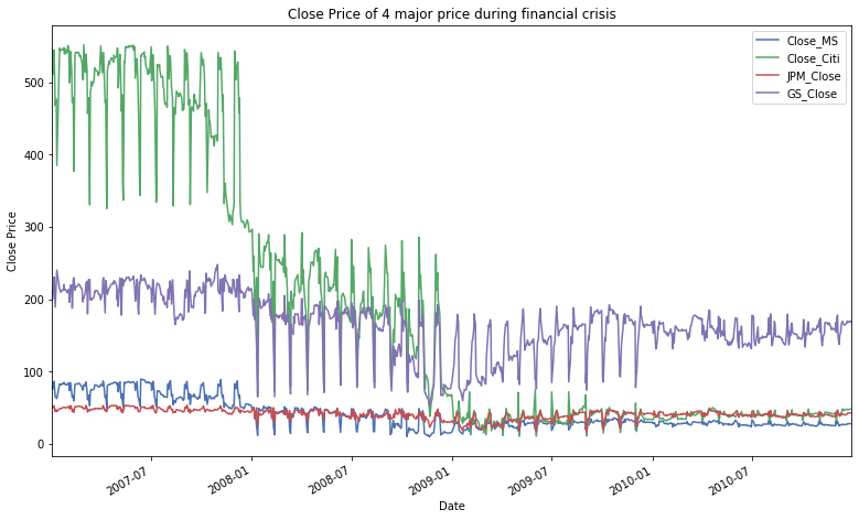
Below Summary explains high volatility of each stock during the time of crisis

df.describe()

	Close_MS	Close_Citi	JPM_Close	GS_Close
count	1007.000000	1007.000000	1007.000000	1007.000000
mean	40.228898	186.092056	40.848590	164.917607
std	20.498821	185.851510	6.746547	40.236383
min	9.200000	10.200000	15.900000	52.000000
25%	26.000000	39.099998	37.730002	144.930001
50%	30.790001	65.199997	41.529999	166.750000
75%	49.979999	292.550003	45.330000	190.285004
max	89.300003	552.500000	53.200001	247.919998

# from 2007 - 2010
df.plot(legend = 'MS',figsize=(13,8))
plt.ylabel("Close Price")
plt.title('Close Price of 4 major price during financial crisis')

Text(0.5, 1.0, 'Close Price of 4 major price during financial crisis')

Quantifying Return (Taking log returns in place of close prices due to high autocorrelation in prices)

df['Lag_MS'] = df['Close_MS'].shift(1)
df['Return_MS'] = (np.log(df['Close_MS']/df['Lag_MS']))*100
df['Lag_Citi'] = df['Close_Citi'].shift(1)
df['Return_Citi'] = (np.log(df['Close_Citi']/df['Lag_Citi']))*100
df['Lag_JPM'] = df['JPM_Close'].shift(1)
df['Return_JPM'] = (np.log(df['JPM_Close']/df['Lag_JPM']))*100
df['Lag_GS'] = df['GS_Close'].shift(1)
df['Return_GS'] = (np.log(df['GS_Close']/df['Lag_GS']))*100

df1 = df.drop(['Lag_Citi','Lag_MS','Lag_JPM','Lag_GS'],axis=1)

df2 = df1.drop(['Close_MS','Close_Citi','GS_Close','JPM_Close'],axis=1)

df3 = df2.copy()

df3.head(10)

	Return_MS	Return_Citi	Return_JPM	Return_GS
Date
2007-03-01	NaN	NaN	NaN	NaN
2007-04-01	0.354677	-0.344488	0.249323	-0.936011
2007-05-01	-1.290186	-0.528084	-0.833508	0.100526
2007-08-01	0.604153	0.509924	0.334239	2.323950
2007-09-01	-0.233824	-0.875756	-0.417976	0.171652
2007-10-01	0.503898	-0.809576	0.730307	1.955471
2007-11-01	0.975978	0.073873	0.435646	1.795331
2007-12-01	0.593112	0.386915	-0.664590	0.990921
2007-01-16	-0.302170	0.714620	0.830046	-0.187104
2007-01-17	-0.278810	-0.696226	0.082630	-0.168689

df3.describe()

	Return_MS	Return_Citi	Return_JPM	Return_GS
count	1006.000000	1006.000000	1006.000000	1006.000000
mean	-0.108756	-0.243700	-0.012875	-0.017902
std	5.008769	5.580447	3.865965	3.441285
min	-29.965820	-49.469624	-23.227805	-21.022262
25%	-1.735934	-1.991310	-1.498332	-1.418094
50%	-0.043817	-0.203060	-0.072195	-0.054054
75%	1.598136	1.576655	1.400192	1.556280
max	62.585004	45.631619	22.391712	23.481773

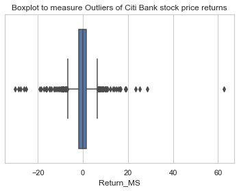
sns.set(style="whitegrid")
# #plt.figure(figsize=(20, 12))
# plt.xlabel('LogReturn')
# style.use('ggplot')
sns.boxplot(x=df3['Return_MS'])
plt.title('Boxplot to measure Outliers of Citi Bank stock price returns')

Text(0.5, 1.0, 'Boxplot to measure Outliers of Citi Bank stock price returns')

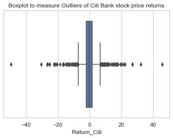
sns.set(style="whitegrid")
sns.boxplot(x=df3['Return_Citi'])
plt.title('Boxplot to measure Outliers of Citi Bank stock price returns')

Text(0.5, 1.0, 'Boxplot to measure Outliers of Citi Bank stock price returns')

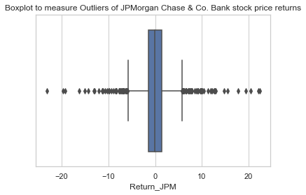
sns.set(style="whitegrid")
sns.boxplot(x=df3['Return_JPM'])
plt.title('Boxplot to measure Outliers of JPMorgan Chase & Co. Bank stock price returns')

Text(0.5, 1.0, 'Boxplot to measure Outliers of JPMorgan Chase & Co. Bank stock price returns')

sns.set(style="whitegrid")
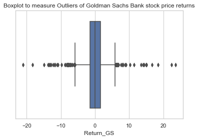
sns.boxplot(x=df3['Return_GS'])
plt.title('Boxplot to measure Outliers of Goldman Sachs Bank stock price returns')

Text(0.5, 1.0, 'Boxplot to measure Outliers of Goldman Sachs Bank stock price returns')

Considering equal weightage to each asset in a portfolio

returns = df3.dropna(axis=0)

Allocation of 25% of our Investment in each of the security

w = (0.25,0.25,0.25,0.25)

# Multilying weight vector with returns vector to calculate portfolio returns
portfolio_returns = returns.dot(w)

portfolio_returns.head(10)

Date
2007-04-01   -0.169125
2007-05-01   -0.637813
2007-08-01    0.943067
2007-09-01   -0.338976
2007-10-01    0.595025
2007-11-01    0.820207
2007-12-01    0.326589
2007-01-16    0.263848
2007-01-17   -0.265274
2007-01-18   -0.922285
dtype: float64

losses = -1*portfolio_returns

losses.head(10)

Date
2007-04-01    0.169125
2007-05-01    0.637813
2007-08-01   -0.943067
2007-09-01    0.338976
2007-10-01   -0.595025
2007-11-01   -0.820207
2007-12-01   -0.326589
2007-01-16   -0.263848
2007-01-17    0.265274
2007-01-18    0.922285
dtype: float64

-ve returns are losses and +ve returns a are profit

Pandas Series Object to Pandas Dataframe

portfolio_returns_new = pd.Series(portfolio_returns)
print (portfolio_returns_new)

Date
2007-04-01   -0.169125
2007-05-01   -0.637813
2007-08-01    0.943067
2007-09-01   -0.338976
2007-10-01    0.595025
                ...   
2010-12-23   -0.600600
2010-12-27    1.245777
2010-12-28    0.058732
2010-12-29   -0.776881
2010-12-30   -0.082041
Length: 1006, dtype: float64

df = portfolio_returns_new.to_frame()

df = df.rename(columns={0: "returns"})

df.head(10)

	returns
Date
2007-04-01	-0.169125
2007-05-01	-0.637813
2007-08-01	0.943067
2007-09-01	-0.338976
2007-10-01	0.595025
2007-11-01	0.820207
2007-12-01	0.326589
2007-01-16	0.263848
2007-01-17	-0.265274
2007-01-18	-0.922285

portfolio_returns.plot(color='red').set_ylabel("Daily Return, %")
plt.show()

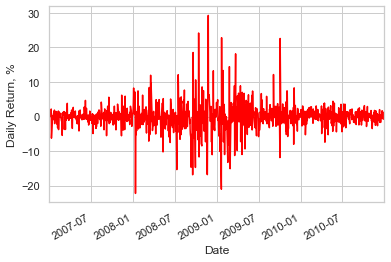
Above graph shows very high volatility from July 2008 to July 2009

The asset prices plot shows how the global financial crisis created a loss in confidence in investment banks from September 2008 There was an event during September that precipitated this decline. The ‘spikiness’ of portfolio returns indicates how uncertain and volatile asset returns became.

portfolio_returns_percent = portfolio_returns*100

VaR using Variance Covariance (Parametric Estimation)

The parametric method, also known as the variance-covariance method, is a risk management technique for calculating the value at risk (VaR) of a portfolio of assets. The value at risk is a statistical risk management technique measuring the maximum loss that an investment portfolio is likely to face within a specified time frame with a certain degree of confidence. The variance-covariance method used to calculate the value at risk identifies the mean, or expected value, and standard deviation of an investment portfolio.

covar = df3.cov()

Correlation in Percentage

print(covar)

             Return_MS  Return_Citi  Return_JPM  Return_GS
Return_MS    25.087771    16.949962   12.411611  13.923230
Return_Citi  16.949962    31.141387   15.314959  12.128333
Return_JPM   12.411611    15.314959   14.945687   9.666014
Return_GS    13.923230    12.128333    9.666014  11.842443

# Annualize the covariance using 252 trading days per year
covar_ann = covar*252

print(covar_ann)

               Return_MS  Return_Citi   Return_JPM    Return_GS
Return_MS    6322.118322  4271.390381  3127.726038  3508.654003
Return_Citi  4271.390381  7847.629460  3859.369779  3056.339857
Return_JPM   3127.726038  3859.369779  3766.313007  2435.835409
Return_GS    3508.654003  3056.339857  2435.835409  2984.295634

portfolio_variance = np.transpose(w)@covar_ann@w

portfolio_volatility = np.sqrt(portfolio_variance)

Annual Portfolio Volatliltiy of 61%

The volatility of a portfolio of stocks is a measure of how wildly the total value of all the stocks in that portfolio appreciates or declines.

print(portfolio_volatility)

61.96722286680826

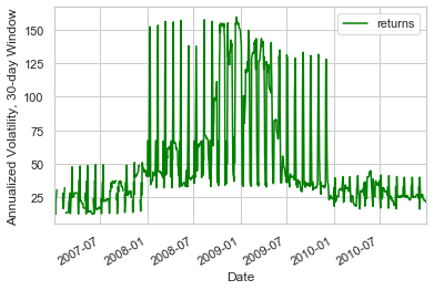
30 Day Rolling Volatility

windowed = df.rolling(30)

volatility = windowed.std()*np.sqrt(252)

volatility.plot(color = 'green').set_ylabel("Annualized Volatility, 30-day Window")

Text(0, 0.5, 'Annualized Volatility, 30-day Window')

df.head(10)

	returns
Date
2007-04-01	-0.169125
2007-05-01	-0.637813
2007-08-01	0.943067
2007-09-01	-0.338976
2007-10-01	0.595025
2007-11-01	0.820207
2007-12-01	0.326589
2007-01-16	0.263848
2007-01-17	-0.265274
2007-01-18	-0.922285

Risk Factors

Variables or events that drive portfolio return and volatility

Two types of risk factors are: 1. Systematic Risk 2. Idisyncratic Risk

Systematic Risk

Systematic risk is inherent to the market as a whole, reflecting the impact of economic, geo-political and financial factors. This type of risk is distinguished from unsystematic risk, which impacts a specific industry or security. Investors can somewhat mitigate the impact of systematic risk by building a diversified portfolio. Ex: interest rate changes, inflation, recessions, and wars, among other major changes.

Idiosyncratic Risk

Idiosyncratic risk refers to the inherent factors that can negatively impact individual securities or a very specific group of assets. The opposite of Idiosyncratic risk is a systematic risk, which refers to broader trends that impact the overall financial system or a very broad market. Idiosyncratic risk can generally be mitigated in an investment portfolio through the use of diversification Idiosyncratic risk is a type of investment risk that is endemic to an individual asset (like a particular company’s stock), or a group of assets (like a particular sector’s stocks), or in some cases, a very specific asset class (like collateralized mortgage obligations).

Idiosyncratic Risk vs. Systematic Risk

While idiosyncratic risk is, by definition, irregular and unpredictable, studying a company or industry can help an investor to identify and anticipate—in a general way—its idiosyncratic risks. Idiosyncratic risk is also highly individual, even unique in some cases. It can, therefore, be substantially mitigated or eliminated from a portfolio by using adequate diversification. Proper asset allocation, along with hedging strategies, can minimize its negative impact on an investment portfolio by diversification or hedging. In contrast, systematic risk cannot be mitigated just by adding more assets to an investment portfolio. This market risk cannot be eliminated by adding stocks of various sectors to one’s holdings. These broader types of risk reflect the macroeconomic factors that affect not just a single asset but other assets like it and greater markets and economies as well.

Factor Models

Factor models assess on which risk factors asset returns or volatility are mostly dependent. We can model theses factors using : 1. Ordinary Least Square - Regression Model - dependent variable - Asset returns/volatility independent variable - risk factors 2. Fama French Model - combination of market risk and idiosyncratic risk (firm size and value)

Considering MBS(Mortgage Backed Security) 90 days mortgage Delinquency as a risk factor which caused the bankcruptcy of Lehman Brothers. Risk factor delinquency rate was highly correlated with the returns.

Risk factor models often rely upon data that is of different frequencies. A typical example is when using quarterly macroeconomic data, such as prices, unemployment rates. here also delinquency rate is taken for 90 days (1 Q) so sampling returns for quarter

returns_avg = df.resample('Q').mean()

returns_avg.tail()

	returns
Date
2009-12-31	-0.028065
2010-03-31	0.269598
2010-06-30	-0.182155
2010-09-30	0.090613
2010-12-31	-0.056955

# Now convert daily returns to weekly minimum returns
returns_min = df.resample('Q').min()
returns_min.head()

	returns
Date
2007-03-31	-6.233800
2007-06-30	-4.161445
2007-09-30	-5.513566
2007-12-31	-5.545354
2008-03-31	-22.216434

delin = pd.read_csv("Delinq_rate.csv")

returns_avg.describe()

	returns
count	16.000000
mean	-0.097230
std	0.367616
min	-0.718012
25%	-0.228185
50%	-0.064064
75%	0.082071
max	0.512064

delin.describe()

	Delinq_Rate
count	16.000000
mean	0.073975
std	0.033431
min	0.023100
25%	0.042025
50%	0.082700
75%	0.103525
max	0.115400

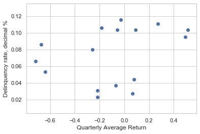
plt.scatter(returns_avg,delin['Delinq_Rate'])
plt.xlabel("Quarterly Average Return")
plt.ylabel("Delinquency rate, decimal %")

Text(0, 0.5, 'Delinquency rate, decimal %')

plt.scatter(returns_min,delin['Delinq_Rate'])
plt.xlabel("Quarterly Min Return")
plt.ylabel("Delinquency rate, decimal %")

Text(0, 0.5, 'Delinquency rate, decimal %')

Initial assessment indicates that there is little correlation between average returns and mortgage delinquencies, but a stronger negative correlation exists between minimum returns and delinquency. In the following exercises we’ll quantify this using least-squares regression.

delin.head()

	Date	Delinq_Rate
0	31-03-2007	0.0231
1	30-06-2007	0.0271
2	30-09-2007	0.0309
3	31-12-2007	0.0367
4	31-03-2008	0.0438

delin['Date'] = pd.to_datetime(delin['Date'])
delin = delin.set_index('Date')

delin.head()

	Delinq_Rate
Date
2007-03-31	0.0231
2007-06-30	0.0271
2007-09-30	0.0309
2007-12-31	0.0367
2008-03-31	0.0438

regression = sm.OLS(returns_avg,delin['Delinq_Rate']).fit()

print(regression.summary())

                                 OLS Regression Results                                
=======================================================================================
Dep. Variable:                returns   R-squared (uncentered):                   0.015
Model:                            OLS   Adj. R-squared (uncentered):             -0.051
Method:                 Least Squares   F-statistic:                             0.2271
Date:                Sat, 25 Jul 2020   Prob (F-statistic):                       0.641
Time:                        08:04:12   Log-Likelihood:                         -6.6308
No. Observations:                  16   AIC:                                      15.26
Df Residuals:                      15   BIC:                                      16.03
Df Model:                           1                                                  
Covariance Type:            nonrobust                                                  
===============================================================================
                  coef    std err          t      P>|t|      [0.025      0.975]
-------------------------------------------------------------------------------
Delinq_Rate    -0.5580      1.171     -0.476      0.641      -3.054       1.938
==============================================================================
Omnibus:                        0.056   Durbin-Watson:                   1.468
Prob(Omnibus):                  0.973   Jarque-Bera (JB):                0.252
Skew:                          -0.099   Prob(JB):                        0.882
Kurtosis:                       2.417   Cond. No.                         1.00
==============================================================================

Warnings:
[1] Standard Errors assume that the covariance matrix of the errors is correctly specified.


C:\Users\TAN\Anaconda3\lib\site-packages\scipy\stats\stats.py:1535: UserWarning:

kurtosistest only valid for n>=20 ... continuing anyway, n=16

regression_qmin = sm.OLS(returns_min,delin['Delinq_Rate']).fit()

print(regression_qmin.summary())

                                 OLS Regression Results                                
=======================================================================================
Dep. Variable:                returns   R-squared (uncentered):                   0.594
Model:                            OLS   Adj. R-squared (uncentered):              0.567
Method:                 Least Squares   F-statistic:                              21.92
Date:                Sat, 25 Jul 2020   Prob (F-statistic):                    0.000295
Time:                        08:04:15   Log-Likelihood:                         -54.585
No. Observations:                  16   AIC:                                      111.2
Df Residuals:                      15   BIC:                                      111.9
Df Model:                           1                                                  
Covariance Type:            nonrobust                                                  
===============================================================================
                  coef    std err          t      P>|t|      [0.025      0.975]
-------------------------------------------------------------------------------
Delinq_Rate  -109.8156     23.454     -4.682      0.000    -159.808     -59.824
==============================================================================
Omnibus:                        0.853   Durbin-Watson:                   0.828
Prob(Omnibus):                  0.653   Jarque-Bera (JB):                0.718
Skew:                          -0.452   Prob(JB):                        0.698
Kurtosis:                       2.489   Cond. No.                         1.00
==============================================================================

Warnings:
[1] Standard Errors assume that the covariance matrix of the errors is correctly specified.

# Now convert daily returns to weekly minimum returns
returns_vol = df.resample('Q').std()
returns_vol.head()

	returns
Date
2007-03-31	1.787018
2007-06-30	1.434462
2007-09-30	1.909144
2007-12-31	2.157466
2008-03-31	4.694626

regression_vol = sm.OLS(returns_vol,delin['Delinq_Rate']).fit()

print(regression_vol.summary())

                                 OLS Regression Results                                
=======================================================================================
Dep. Variable:                returns   R-squared (uncentered):                   0.657
Model:                            OLS   Adj. R-squared (uncentered):              0.634
Method:                 Least Squares   F-statistic:                              28.68
Date:                Sat, 25 Jul 2020   Prob (F-statistic):                    8.01e-05
Time:                        08:04:18   Log-Likelihood:                         -35.971
No. Observations:                  16   AIC:                                      73.94
Df Residuals:                      15   BIC:                                      74.71
Df Model:                           1                                                  
Covariance Type:            nonrobust                                                  
===============================================================================
                  coef    std err          t      P>|t|      [0.025      0.975]
-------------------------------------------------------------------------------
Delinq_Rate    39.2452      7.328      5.356      0.000      23.627      54.864
==============================================================================
Omnibus:                        1.168   Durbin-Watson:                   0.517
Prob(Omnibus):                  0.558   Jarque-Bera (JB):                0.832
Skew:                           0.215   Prob(JB):                        0.660
Kurtosis:                       1.969   Cond. No.                         1.00
==============================================================================

Warnings:
[1] Standard Errors assume that the covariance matrix of the errors is correctly specified.

As seen from the regressions, mortgage delinquencies are acting as a systematic risk factor for both minimum quarterly returns and average volatility of returns, but not for average quarterly returns. The R-squared goodness of fit isn’t high in any case, but a model with more factors would likely generate greater explanatory power.

R-Squared is a statistical measure of fit that indicates how much variation of a dependent variable is explained by the independent variable(s) in a regression model.

Modern Portfolio Theory

What maximum return an investor can expect as per given risk apetite calculated from the portfolio volatility

Eficient Portfolio

portfolio with weights generating highest expected return for given level of risk

Efficient Frontier

Locus of (risk,return) pairs created by efficient portfolio

# pip install pyportfolioopt

# Compute the annualized average historical return
mean_returns = mean_historical_return(df4, frequency = 252)

# Plot the annualized average historical return
plt.plot(mean_returns, linestyle = 'None', marker = 'o')
plt.show()

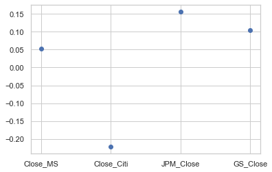
mean_returns.head()

Close_MS      0.051932
Close_Citi   -0.222364
JPM_Close     0.156725
GS_Close      0.104710
dtype: float64

The average historical return is usually available as a proxy for expected returns, but is not always accurate–a more thorough estimate of expected returns requires an assumption about the return distribution, which we’ll discuss in the context of Loss Distributions later in the course.

df4.head(10)

	Close_MS	Close_Citi	JPM_Close	GS_Close
Date
2007-03-01	81.620003	552.500000	48.070000	200.720001
2007-04-01	81.910004	550.599976	48.189999	198.850006
2007-05-01	80.860001	547.700012	47.790001	199.050003
2007-08-01	81.349998	550.500000	47.950001	203.729996
2007-09-01	81.160004	545.700012	47.750000	204.080002
2007-10-01	81.570000	541.299988	48.099998	208.110001
2007-11-01	82.370003	541.700012	48.310001	211.880005
2007-12-01	82.860001	543.799988	47.990002	213.990005
2007-01-16	82.610001	547.700012	48.389999	213.589996
2007-01-17	82.379997	543.900024	48.430000	213.229996

# Import the CovarianceShrinkage object, it reduces/shrinks the errors/residuals while calculating the covariance matrix
# Create the CovarianceShrinkage instance variable
cs = CovarianceShrinkage(df4)

# Difference in calculating covariance matrix through covariance shrinkage and through sample cov() method
# Compute the sample covariance matrix of returns
sample_cov = df4.pct_change().cov() * 252

# Compute the efficient covariance matrix of returns
e_cov = cs.ledoit_wolf()

# Display both the sample covariance_matrix and the efficient e_cov estimate
print("Sample Covariance Matrix\n", sample_cov, "\n")
print("Efficient Covariance Matrix\n", e_cov, "\n")

Sample Covariance Matrix
             Close_MS  Close_Citi  JPM_Close  GS_Close
Close_MS    0.717102    0.450956   0.319404  0.372737
Close_Citi  0.450956    0.796039   0.398215  0.320531
JPM_Close   0.319404    0.398215   0.384847  0.247412
GS_Close    0.372737    0.320531   0.247412  0.304432 

Efficient Covariance Matrix
             Close_MS  Close_Citi  JPM_Close  GS_Close
Close_MS    0.707324    0.425953   0.301695  0.352071
Close_Citi  0.425953    0.781884   0.376136  0.302760
JPM_Close   0.301695    0.376136   0.393490  0.233695
GS_Close    0.352071    0.302760   0.233695  0.317534 

Although the differences between the sample covariance and the efficient covariance (found by shrinking errors) may seem small, they have a huge impact on estimation of the optimal portfolio weights and the generation of the efficient frontier. Practitioners generally use some form of efficient covariance for Modern Portfolio Theory.

# Create a dictionary of time periods (or 'epochs')
epochs = { 'during' : {'start': '1-1-2007', 'end': '31-12-2008'},
           'after'  : {'start': '1-1-2009', 'end': '31-12-2010'}
         }

# Compute the efficient covariance for each epoch
e_cov = {}
for x in epochs.keys():
    sub_price = df4.loc[epochs[x]['start']:epochs[x]['end']]
    e_cov[x] = CovarianceShrinkage(sub_price).ledoit_wolf()

# Display the efficient covariance matrices for all epochs
print("Efficient Covariance Matrices\n", e_cov)

Efficient Covariance Matrices
 {'during':             Close_MS  Close_Citi  JPM_Close  GS_Close
Close_MS    0.994390    0.465336   0.298613  0.434874
Close_Citi  0.465336    0.713035   0.364848  0.323977
JPM_Close   0.298613    0.364848   0.422516  0.224668
GS_Close    0.434874    0.323977   0.224668  0.408773, 'after':             Close_MS  Close_Citi  JPM_Close  GS_Close
Close_MS    0.388839    0.344939   0.279727  0.231624
Close_Citi  0.344939    0.841156   0.356788  0.252684
JPM_Close   0.279727    0.356788   0.382494  0.223740
GS_Close    0.231624    0.252684   0.223740  0.244539}

df3.head()

	Return_MS	Return_Citi	Return_JPM	Return_GS
Date
2007-03-01	NaN	NaN	NaN	NaN
2007-04-01	0.354677	-0.344488	0.249323	-0.936011
2007-05-01	-1.290186	-0.528084	-0.833508	0.100526
2007-08-01	0.604153	0.509924	0.334239	2.323950
2007-09-01	-0.233824	-0.875756	-0.417976	0.171652

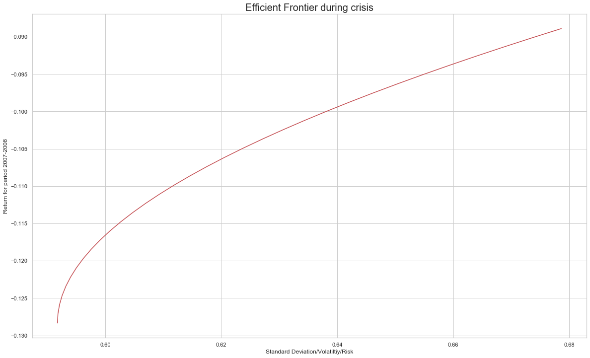
Great! The breakdown of the 2007 - 2010 period into sub-periods shows how the portfolio’s risk increased during the crisis , and this changed the risk-return trade-off after the crisis. For future reference, also note that although we used a loop in this exercise, a dictionary comprehension could also have been used to create the efficient covariance matrix.

# Create a dictionary of time periods (or 'epochs')
epochs = { 'during' : {'start': '1-1-2007', 'end': '31-12-2008'}}

# Compute the efficient covariance for each epoch
e_cov_during = {}
for x in epochs.keys():
    sub_price = df4.loc[epochs[x]['start']:epochs[x]['end']]
    e_cov_during[x] = CovarianceShrinkage(sub_price).ledoit_wolf()

# Display the efficient covariance matrices for all epochs
print("Efficient Covariance Matrices\n", e_cov_during)

Efficient Covariance Matrices
 {'during':             Close_MS  Close_Citi  JPM_Close  GS_Close
Close_MS    0.994390    0.465336   0.298613  0.434874
Close_Citi  0.465336    0.713035   0.364848  0.323977
JPM_Close   0.298613    0.364848   0.422516  0.224668
GS_Close    0.434874    0.323977   0.224668  0.408773}

Efficient Frontier Using CLA Algorithm

Compute many efficient portfolios for different levels of risk efficient frontier: locus of (risk, return) pairs created by efficient portfolios PyPortfolioOpt library: optimized tools for MPT EfficientFrontier class: generates one optimal portfolio at a time Constrained Line Algorithm ( CLA ) class: generates the entire efficient frontier Requires covariance matrix of returns Requires proxy for expected future returns: mean historical returns

df4.head()

	Close_MS	Close_Citi	JPM_Close	GS_Close
Date
2007-03-01	81.620003	552.500000	48.070000	200.720001
2007-04-01	81.910004	550.599976	48.189999	198.850006
2007-05-01	80.860001	547.700012	47.790001	199.050003
2007-08-01	81.349998	550.500000	47.950001	203.729996
2007-09-01	81.160004	545.700012	47.750000	204.080002

df3.head()

	Return_MS	Return_Citi	Return_JPM	Return_GS
Date
2007-03-01	NaN	NaN	NaN	NaN
2007-04-01	0.354677	-0.344488	0.249323	-0.936011
2007-05-01	-1.290186	-0.528084	-0.833508	0.100526
2007-08-01	0.604153	0.509924	0.334239	2.323950
2007-09-01	-0.233824	-0.875756	-0.417976	0.171652

df6=df3.loc['2007-03-01':'2008-12-31']

df7=df4.loc['2007-03-01':'2008-12-31']

e_cov_during = np.array(CovarianceShrinkage(df7).ledoit_wolf())

type(e_cov_during)

numpy.ndarray

returns_during = np.array(df6.mean())

efficient_portfolio_during = CLA(returns_during, e_cov_during)

print(efficient_portfolio_during.min_volatility())

{0: 0.0, 1: 0.0, 2: 0.4814250629859924, 3: 0.5185749370140076}

# Compute the efficient frontier
(ret, vol, weights) = efficient_portfolio_during.efficient_frontier()

plt.figure(figsize=(20,12))
plt.xlabel('Standard Deviation/Volatiltiy/Risk')
plt.ylabel('Return for period 2007-2008')
plt.title('Efficient Frontier during crisis',size=20)
plt.plot(vol,ret,c='r')

[<matplotlib.lines.Line2D at 0x27255455ac8>]

df9=df4.loc['2009-01-01':'2010-12-31']  # for covariance matrix (prices)
df10=df3.loc['2009-01-01':'2010-12-31'] # returns

returns_after = np.array(df10.mean())
print(returns_after)

[ 0.1059442  -0.06826069  0.05808973  0.13645525]

e_cov_after = np.array(CovarianceShrinkage(df9).ledoit_wolf())
efficient_portfolio_after = CLA(returns_after, e_cov_after)
(ret, vol, weights) = efficient_portfolio_after.efficient_frontier()
# Add the frontier to the plot showing the 'before' and 'after' frontiers

plt.figure(figsize=(20,12))
plt.xlabel('Standard Deviation/Volatiltiy/Risk')
plt.ylabel('Return for period 2009-2010')
plt.title('Efficient Frontier after crisis',size=20)
plt.plot(vol,ret,c='g')

[<matplotlib.lines.Line2D at 0x27255a9a5f8>]

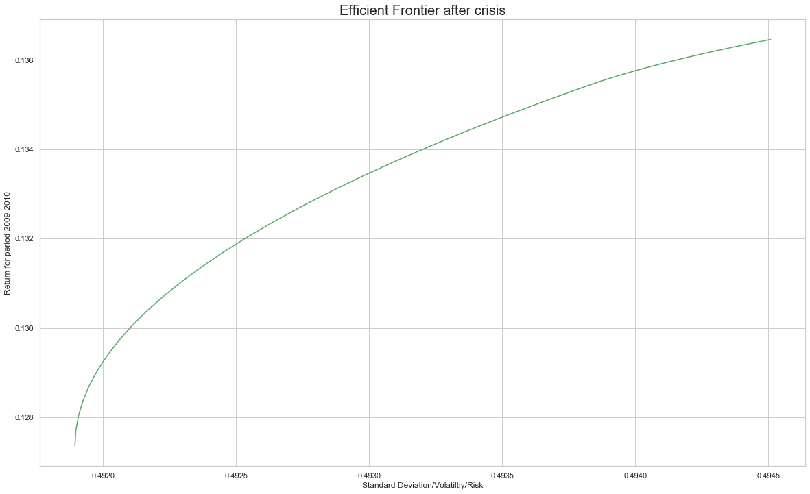
## Risk reduced after crisis

Portfolio Optimization

df_returns = df1[['Return_MS','Return_Citi','Return_JPM','Return_GS']]

df_returns.head(10)

	Return_MS	Return_Citi	Return_JPM	Return_GS
Date
2007-03-01	NaN	NaN	NaN	NaN
2007-04-01	0.354677	-0.344488	0.249323	-0.936011
2007-05-01	-1.290186	-0.528084	-0.833508	0.100526
2007-08-01	0.604153	0.509924	0.334239	2.323950
2007-09-01	-0.233824	-0.875756	-0.417976	0.171652
2007-10-01	0.503898	-0.809576	0.730307	1.955471
2007-11-01	0.975978	0.073873	0.435646	1.795331
2007-12-01	0.593112	0.386915	-0.664590	0.990921
2007-01-16	-0.302170	0.714620	0.830046	-0.187104
2007-01-17	-0.278810	-0.696226	0.082630	-0.168689

df_returns.hist(bins=100,figsize=(12,8))
plt.tight_layout()

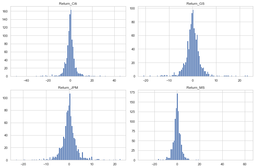
df_returns.mean()

Return_MS     -0.108756
Return_Citi   -0.243700
Return_JPM    -0.012875
Return_GS     -0.017902
dtype: float64

df_returns.cov()*252

	Return_MS	Return_Citi	Return_JPM	Return_GS
Return_MS	6322.118322	4271.390381	3127.726038	3508.654003
Return_Citi	4271.390381	7847.629460	3859.369779	3056.339857
Return_JPM	3127.726038	3859.369779	3766.313007	2435.835409
Return_GS	3508.654003	3056.339857	2435.835409	2984.295634

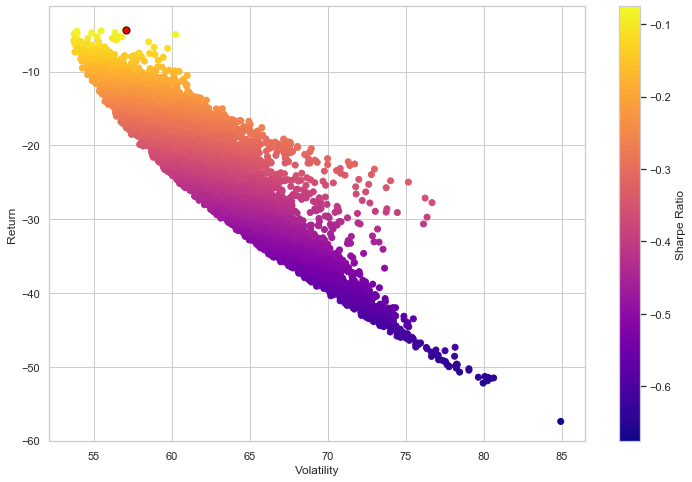
Portfolio Optimization using Monte Carlo Simulation (Random Weights)

np.random.seed(101)
print(df1.columns)
rand_weights = np.array(np.random.rand(4))
print('Random Weights : ',rand_weights)
## To make sum of random weights equal to 1 , divide each random generated weight by sum
print('Rebalance')
weights = rand_weights/np.sum(rand_weights)
print(weights)

Index(['Close_MS', 'Close_Citi', 'JPM_Close', 'GS_Close', 'Return_MS',
       'Return_Citi', 'Return_JPM', 'Return_GS'],
      dtype='object')
Random Weights :  [0.51639863 0.57066759 0.02847423 0.17152166]
Rebalance
[0.40122278 0.44338777 0.02212343 0.13326603]

## Yearly portfolio expected return
exp_ret = np.sum(df_returns.mean()*weights*252)
exp_ret

-38.898628588158786

## Portfolio Volatility Yearly
exp_vol = np.sqrt(np.dot(weights.T,np.dot(df_returns.cov()*252,weights)))
exp_vol

70.83152895453853

## Sharpe Ratio
sr = exp_ret/exp_vol
print('Sharpe Ratio :',sr)

Sharpe Ratio : -0.5491710988354481

## Final code for monte carlo
np.random.seed(101)
num_ports = 10000
all_weights = np.zeros((num_ports,len(df_returns.columns)))
ret_arr = np.zeros(num_ports)
vol_arr = np.zeros(num_ports)
sharpe_arr = np.zeros(num_ports)

for ind in range(num_ports):
    rand_weights = np.array(np.random.rand(4))
    ## To make sum of random weights equal to 1 , divide each random generated weight by sum
    weights = rand_weights/np.sum(rand_weights)
    all_weights[ind,:] = weights
    ## Yearly portfolio expected return
    ret_arr[ind] = np.sum(df_returns.mean()*weights*252)
    ## Portfolio Volatility Yearly
    vol_arr[ind] = np.sqrt(np.dot(weights.T,np.dot(df_returns.cov()*252,weights)))
    ## Sharpe Ratio
    sharpe_arr[ind] = ret_arr[ind]/vol_arr[ind]

sharpe_arr.max()

sharpe_arr.argmax()

7872

all_weights[7872,:]

array([0.01225268, 0.00812669, 0.74934034, 0.2302803 ])

max_sr_ret = ret_arr[7872]
max_sr_vol = vol_arr[7872]

plt.figure(figsize=(12,8))
plt.scatter(vol_arr,ret_arr,c=sharpe_arr,cmap='plasma')
plt.colorbar(label='Sharpe Ratio')
plt.xlabel('Volatility')
plt.ylabel('Return')
plt.scatter(max_sr_vol,max_sr_ret,c='red',s=50,edgecolors='black')

<matplotlib.collections.PathCollection at 0x27253fcd630>

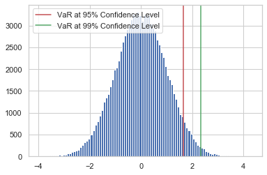
Var(Value at Risk) of a Normal Distribution

# Var of a Normal Distribution
# Create the VaR measure at the 95% confidence level using norm.ppf()
VaR_95 = norm.ppf(0.95)

# Create the VaR meaasure at the 5% significance level using numpy.quantile()
draws = norm.rvs(size = 100000)
VaR_99 = np.quantile(draws, 0.99)

# Compare the 95% and 99% VaR
print("95% VaR: ", VaR_95, "; 99% VaR: ", VaR_99)

# Plot the normal distribution histogram and 95% VaR measure
plt.hist(draws, bins = 100)
plt.axvline(x = VaR_95, c='r', label = "VaR at 95% Confidence Level")
plt.axvline(x = VaR_99, c='g', label = "VaR at 99% Confidence Level")

plt.legend(); plt.show()

95% VaR:  1.6448536269514722 ; 99% VaR:  2.317671064617457

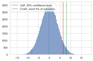
CVAR of a Normal Distribution

losses.head(10)

Date
2007-04-01    0.169125
2007-05-01    0.637813
2007-08-01   -0.943067
2007-09-01    0.338976
2007-10-01   -0.595025
2007-11-01   -0.820207
2007-12-01   -0.326589
2007-01-16   -0.263848
2007-01-17    0.265274
2007-01-18    0.922285
dtype: float64

mean_loss = losses.mean()

mean_loss

0.09580838926126413

std_loss = losses.std()

std_loss

3.903568122449752

# Compute the mean and variance of the portfolio losses
pm = mean_loss
ps = std_loss

# Compute the 95% VaR using the .ppf()
VaR_95 = norm.ppf(0.95, loc = pm, scale = ps)
# Compute the expected tail loss and the CVaR in the worst 5% of cases
tail_loss = norm.expect(lambda x: x, loc = pm, scale = ps, lb = VaR_95)
CVaR_95 = (1 / (1 - 0.95)) * tail_loss

# Plot the normal distribution histogram and add lines for the VaR and CVaR
plt.hist(norm.rvs(size = 100000, loc = pm, scale = ps), bins = 100)
plt.axvline(x = VaR_95, c='r', label = "VaR, 95% confidence level")
plt.axvline(x = CVaR_95, c='g', label = "CVaR, worst 5% of outcomes")
plt.legend(); plt.show()

VaR of Student’s t-distribution

from scipy.stats import t

mu = losses.rolling(30).mean()
sigma = losses.rolling(30).std()

mu

Date
2007-04-01         NaN
2007-05-01         NaN
2007-08-01         NaN
2007-09-01         NaN
2007-10-01         NaN
                ...   
2010-12-23   -0.105515
2010-12-27   -0.175961
2010-12-28   -0.233157
2010-12-29   -0.170770
2010-12-30   -0.219959
Length: 1006, dtype: float64

sigma

Date
2007-04-01         NaN
2007-05-01         NaN
2007-08-01         NaN
2007-09-01         NaN
2007-10-01         NaN
                ...   
2010-12-23    1.425831
2010-12-27    1.428301
2010-12-28    1.386096
2010-12-29    1.388099
2010-12-30    1.350370
Length: 1006, dtype: float64

rolling_parameters = [(29, mu[i], s) for i,s in enumerate(sigma)]
VaR_99 = np.array( [ t.ppf(0.99, *params) 
                    for params in rolling_parameters ] )

# Fit the Student's t distribution to crisis losses
p = t.fit(losses)

# Compute the VaR_99 for the fitted distribution
VaR_99 = t.ppf(0.99, *p)

# Use the fitted parameters and VaR_99 to compute CVaR_99
tail_loss = t.expect( lambda y: y, args = (p[0],), loc = p[1], scale = p[2], lb = VaR_99 )
CVaR_99 = (1 / (1 - 0.99)) * tail_loss
print(CVaR_99)

26.276295920436993

26% Loss (CVaR) on a given portfolio investment during financial crisis

Parametric Estimation VaR

Parameter estimation is the strongest method of VaR estimation because it assumes that the loss distribution class is known. Parameters are estimated to fit data to this distribution, and statistical inference is then made.

Finding best parameters (Theta - Mean and SD) given portfolio data is called Parametric Estimation

In Parameter Estimation VaR, loss distribution is not given, thereby we fit different distribution and with the help of Anderson Darling test we check goodness of fit.

df.head(10)

	returns
Date
2007-04-01	-0.169125
2007-05-01	-0.637813
2007-08-01	0.943067
2007-09-01	-0.338976
2007-10-01	0.595025
2007-11-01	0.820207
2007-12-01	0.326589
2007-01-16	0.263848
2007-01-17	-0.265274
2007-01-18	-0.922285

df_returns = df.dropna(axis=0)

df_returns.head(3)

	returns
Date
2007-04-01	-0.169125
2007-05-01	-0.637813
2007-08-01	0.943067

df_returns.describe()

	returns
count	1006.000000
mean	-0.095808
std	3.903568
min	-22.216434
25%	-1.501236
50%	-0.080673
75%	1.319224
max	29.279192

params = norm.fit(losses)

params

(0.09580838926126402, 3.901627496865014)

VaR_95 = norm.ppf(0.95, *params)

print("VaR_95, Normal distribution: ", VaR_95)

VaR_95, Normal distribution:  6.513414528493276

print("Anderson-Darling test result: ", anderson(losses))

Anderson-Darling test result:  AndersonResult(statistic=38.20183257088229, critical_values=array([0.574, 0.653, 0.784, 0.914, 1.088]), significance_level=array([15. , 10. ,  5. ,  2.5,  1. ]))

The Anderson-Darling test above value of 38.20 exceeds the 99% critical value of 1.088 by a large margin, indicating that the Normal distribution may be a poor choice to represent portfolio losses

## Null Hypothesis - No Skewness

# Test the data for skewness
print("Skewtest result: ", skewtest(losses))

Skewtest result:  SkewtestResult(statistic=-6.655492127945391, pvalue=2.8235366881911988e-11)

# Fit the portfolio loss data to the skew-normal distribution
params = skewnorm.fit(losses)

# Compute the 95% VaR from the fitted distribution, using parameter estimates
VaR_95 = skewnorm.ppf(0.95, *params)
print("VaR_95 from skew-normal: ", VaR_95)

VaR_95 from skew-normal:  6.283943890895702

Losses are not normally distributed as the critical value exceeeds the 99% conidence interval of test statistic value Losses can be skewed

Definition wiki - anderson In many cases (but not all), you can determine a p value for the Anderson-Darling statistic and use that value to help you determine if the test is significant are not. Remember the p (“probability”) value is the probability of getting a result #that is more extreme if the null hypothesis is true. If the p value is low (e.g., <=0.05), you conclude that the data do not follow the normal distribution. Remember that you chose the significance level even though many people just use 0.05 the vast majority of the time. We will look at two different data sets and apply the Anderson-Darling test to both sets.

Note that although the VaR estimate for the Normal distribution from the previous exercise is larger than the skewed Normal distribution estimate, the Anderson-Darling and skewtest results show the Normal distribution estimates cannot be relied upon. Skewness matters for loss distributions, and parameter estimation is one way to quantify this important feature of the financial crisis.

Historical Simulation

EXAMPLE

#weights = [0.25, 0.25, 0.25, 0.25] #portfolio_returns = asset_returns.dot(weights) #losses = - portfolio_returns #VaR_95 = np.quantile(losses, 0.95)

Historical simulation: use past to predict future No distributional assumption required Data about previous losses become simulated losses for tomorrow

VaR_95_HS = np.quantile(losses,0.95)

print(VaR_95_HS)

5.245684561193499

## 5 % Loss with 95% confidence interval

Historical with monte carlo simulation VaR

# Initialize daily cumulative loss for the 4 assets, across N runs
N=10000
daily_loss = np.zeros((4,N))

returns.head()

	Return_MS	Return_Citi	Return_JPM	Return_GS
Date
2007-04-01	0.354677	-0.344488	0.249323	-0.936011
2007-05-01	-1.290186	-0.528084	-0.833508	0.100526
2007-08-01	0.604153	0.509924	0.334239	2.323950
2007-09-01	-0.233824	-0.875756	-0.417976	0.171652
2007-10-01	0.503898	-0.809576	0.730307	1.955471

mu = np.array([returns['Return_MS'].mean(),returns['Return_Citi'].mean(),returns['Return_JPM'].mean(),
               returns['Return_GS'].mean()])

mu

array([-0.1087564 , -0.24369987, -0.01287549, -0.0179018 ])

mu = np.array([[-0.1087564],
      [-0.24369987],
      [-0.01287549],
      [-0.0179018]])

type(mu)

numpy.ndarray

e_cov = returns.cov()

e_cov_1 = np.array(e_cov)

e_cov_1

array([[25.08777112, 16.94996183, 12.41161126, 13.92323017],
       [16.94996183, 31.14138675, 15.31495944, 12.12833277],
       [12.41161126, 15.31495944, 14.94568654,  9.66601353],
       [13.92323017, 12.12833277,  9.66601353, 11.84244299]])

total_steps = 1440

# Create the Monte Carlo simulations for N runs
for n in range(N):
    # Compute simulated path of length total_steps for correlated returns
    correlated_randomness = e_cov @ norm.rvs(size = (4,total_steps))
    # Adjust simulated path by total_steps and mean of portfolio losses
    steps = 1/total_steps
    minute_losses = mu * steps + correlated_randomness * np.sqrt(steps)
    daily_loss[:, n] = minute_losses.sum(axis=1)

losses = weights @ daily_loss
print("Monte Carlo VaR_95 estimate: ", np.quantile(losses, 0.95))

Ordinary Least Square Ordinary least squares (OLS) regression is a statistical method of analysis that estimates the relationship between one or more independent variables and a dependent variable; the method estimates the relationship by minimizing the sum of the squares in the difference between the observed and predicted values of the dependent variable configured as a straight line.

Structural Breaks - Theory

Chow Test = Whether or not a structural break has occured in the data Visualization cannot determine exact structural break in the data Alternative - Time of structural break concides with time of increasing volatility Stochastic Volatility Model : Volatility can be analyzed statistically through the random probability distribution but cannot be predicted precisely

To check if the volatility is non stationary rolling window volatility is calculated

VaR and CVaR estimates that data distribution is same throughout (Stationarity Assumption) but there are structural breaks in between.

So Assume specific points in time for change Break up data into sub-periods Within each sub-period, assume stationarity

Chow TEST: Test for evidence of structural breaks 1. Null hypothesis - No break 2. Requires three OLS regressions 3. Regression for entire period 4. Two regressions, before and after break 5. Collect sum-of-squared residuals 6. Test statistic is distributed according to “F” distribution

Noe sometimes it is not easy to visualize the losses to detect the structural break Sometimes we can use Rolling window volatility to visualize the rolling volatity in the given time period

std() calculates a single value of volatility rolling.std calculates rolling volatility and you can plot and see the structural break

Backtesting Backtesting is the process of applying a trading strategy or analytical method to historical data to see how accurately the strategy or method would have predicted actual results.